"피프틴" 태그가 포함된 인스타그램 게시물 개수 추이와 실제 사용량 비교해보기
솜씨좋은장씨
·2020. 9. 12. 11:20


0. 크롤링에 사용한 코드
[Python] Selenium을 활용하여 인스타그램 크롤링 하기!
이번 글에서는 Python과 Selenium을 활용하여 인스타그램 게시물을 크롤링하는 방법에 대해서 적어보려 합니다. 해당 코드를 활용하여 발생하는 문제는 코드 사용자에게 있음을 알려드립니다. 1. 필
somjang.tistory.com
SOMJANG/Instagram_Crawler
인스타그램 크롤러 (Python, Selenium). Contribute to SOMJANG/Instagram_Crawler development by creating an account on GitHub.
github.com
1. 필요한 라이브러리 import 하기
import pandas as pd
from konlpy.tag import Mecab
import matplotlib.pyplot as plt
import matplotlib
from tqdm import tqdm
from collections import Counter
from PIL import Image
import time
import datetime
import json
import re

mecab = Mecab()
2. 인스타그램 크롤링 데이터 column 정보
- 크롤링한 데이터의 기간 : 2012년 ~ 2020년 8월 중순
- location_info : 게시물 위치정보 이름
- location_href : 게시물 위치정보 url
- upload_id     : 게시자 id
- date_text     : 게시물 게시 날짜 ( 월 일 )
- date_time     : 게시물 게시 날짜 ( datetime 형식 )
- date_title    : 게시물 게시 날짜 ( 년 월 일 )
- main_text     : 게시물 본문
- comment       : 게시물 댓글 ( {댓글 순번:{comment_id:댓글 작성자 id, comment_text:댓글 본문}, ~~ }
- 크롤링 코드 작성은 여기에 사용한 코드는 아니지만 대략적인 작성 방법은 아래의 링크를 참고해주세요.
[Python] 인스타그램 태그를 가져와 워드클라우드 만들기!
1. 주제를 선택한 계기 특정 프랜차이즈에 관련된 최근 키워드를 알려주려면 어떤 것을 참고하면 좋을까 생각하다가 인스타그램에 걸려있는 특정 주제에 대한 여러 태그들을 크롤링하여 그 태��
somjang.tistory.com
3. 크롤링 데이터 불러오기 ( csv 파일 )
- upload_id column과 는 comment의 comment_id는 개인정보로 가렸습니다.
insta_data = pd.read_csv("insta_data_new.csv")
insta_data.head()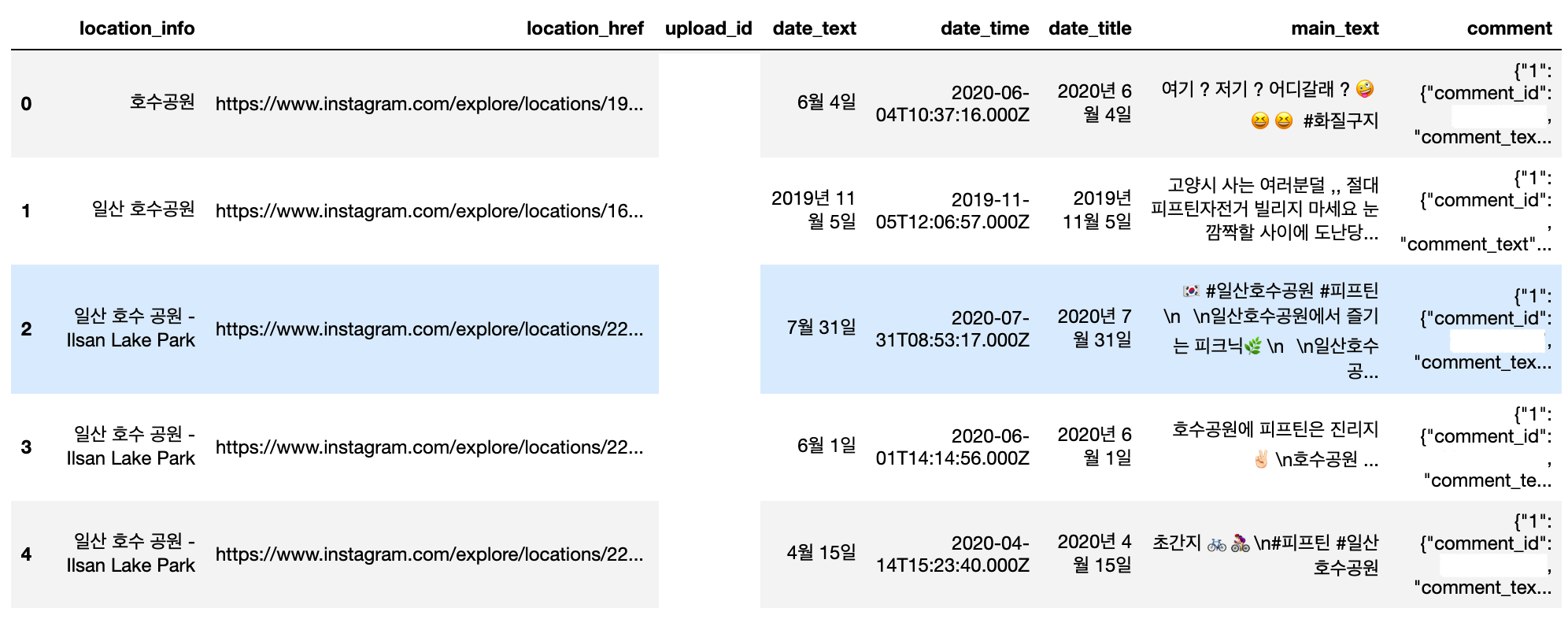
4. 인기 게시물과 같은 중복 게시물 제거
- 중복 데이터 중 본문, 댓글 기준 마지막에 나온 정보 기준
drop_duplicate_data = insta_data.drop_duplicates(['main_text', 'comment'], keep='last')
print(f"중복 제거 전 : {len(insta_data)} -> 중복 제거 후 : {len(drop_duplicate_data)}")
중복 제거 전 : 2010 -> 중복 제거 후 : 1995
중복 제거 이후 15개의 데이터가 제거된 것을 확인할 수 있습니다.
5. 게시물 게시 일자를 기준으로 게시물 개수 추이를 살펴보기
- 방법 1
date_time_strings = list(drop_duplicate_data['date_time'])

date_time_YMD = []

for i in tqdm(range(len(date_time_strings))):
    date_time_YMD.append(date_time_strings[i][:10])
drop_duplicate_data['date_time_YMD'] = date_time_YMD
- 방법 2
drop_duplicate_data['date_time_YMD'] = drop_duplicate_data['date_time'].str.slice(0, 10)먼저 string 형식으로 되어있는 date_time column에서 날짜 정보를 가져옵니다.
date_time column의 각 row 는 년, 월, 일, 시간으로 구성되어 있습니다.
여기서 0~10 index에 있는 년, 월, 일 정보만 추출하고 이를 다시 date_time_YMD에 저장합니다.
위의 방법 2와 같은 방법으로 년, 월 정보도 따로 뽑아 저장합니다.
drop_duplicate_data['date_time_Y'] = drop_duplicate_data['date_time_YMD'].str.slice(0, 4)
drop_duplicate_data['date_time_M'] = drop_duplicate_data['date_time_YMD'].str.slice(5, 7)
6. 일별 게시물 수 시각화
count_by_YMD_Series = drop_duplicate_data['date_time_YMD'].value_counts()
count_by_YMD_df = pd.DataFrame(count_by_YMD_Series)
count_by_YMD_df = count_by_YMD_df.sort_index()
count_by_YMD_df.columns = ['count']
년, 월, 일 정보가 담긴 date_time_YMD column을 기준으로 DataFrame의 value_counts 메소드를 활용하여
각 항목별로 카운팅합니다.
count_by_YMD_df.plot(kind='line', figsize=(100, 20), grid=True)
plt.title('2012-2020 number of instagram post')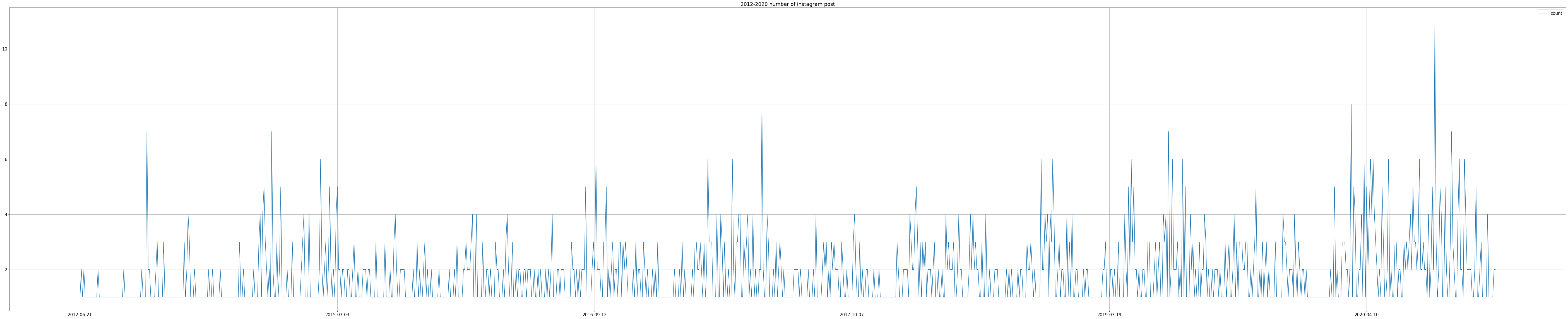
일별로 카운팅한 정보를 그래프로 그려봅니다.
너무 많은 날짜로 인해 한눈에 보기가 어렵습니다.
7. 각 년도별 게시물 수 시각화
이번엔 년도 기준으로 카운팅하고 정렬해봅니다.
drop_duplicate_data['date_time_Y'].value_counts().sort_index()2012 3
2013 11
2014 131
2015 272
2016 301
2017 306
2018 293
2019 336
2020 342
Name: date_time_Y, dtype: int64이를 그래프로 시각화 해봅니다.
plt.figure(figsize=(20, 5))
drop_duplicate_data['date_time_Y'].value_counts().sort_index().plot(grid=True)
drop_duplicate_data['date_time_Y'].value_counts().sort_index().plot(kind='bar', grid=True)
plt.title("The number of Instagram posts 2012-2020")
plt.xticks(rotation=45)
이를 보면 2013년 이후로 대체적으로 게시물 수가 증가하고 있는 것을 볼 수 있습니다.
8. 실제 자전거 사용 현황과 연관이 있는지 확인해보기
- 사용 데이터 : 01.운영이력.csv
COMPAS
COMPAS
compas.lh.or.kr
bike_data = pd.read_csv("../goyang_bike_data/01.운영이력.csv")
bike_data.head()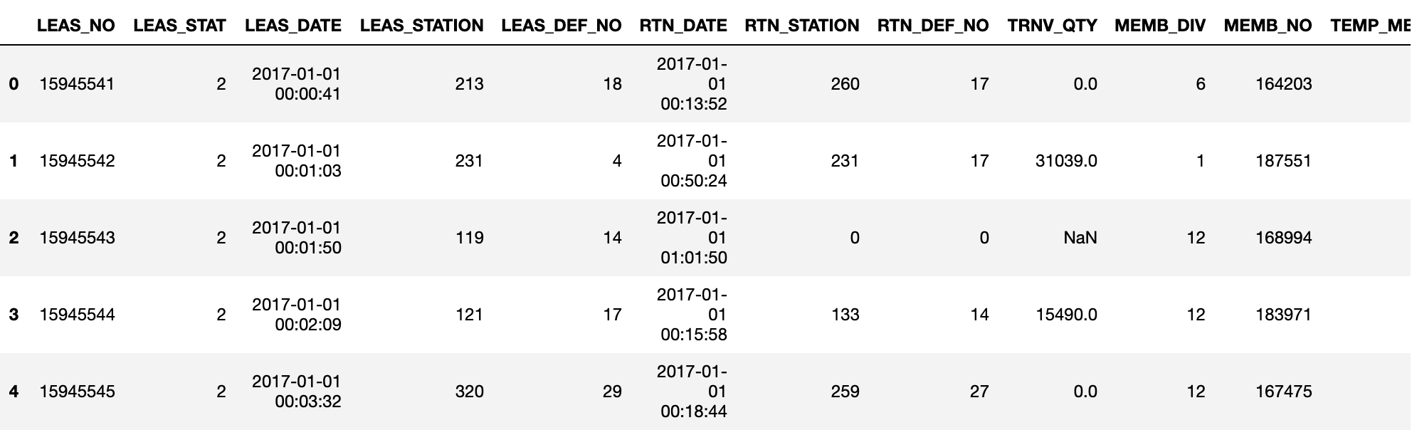
bike_data['LEAS_YM'] = bike_data['LEAS_DATE'].str.slice(0, 7)년월일시분초 데이터가 있는 LEAS_DATE 에서 년월 정보만 추출합니다.
bike_month_usage_df = pd.DataFrame(bike_data['LEAS_YM'].value_counts().sort_index())
bike_dates = bike_month_usage_df.index
bike_month_usage_df['YM'] = bike_dates
bike_month_usage_df['M'] = bike_month_usage_df['YM'].str.slice(5, 7)
bike_month_usage_df['Y'] = bike_month_usage_df['YM'].str.slice(0, 4)
bike_month_usage_df.head()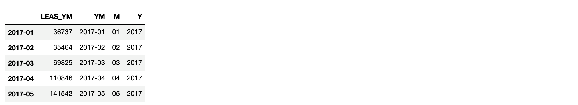
년-월을 기준으로 카운팅하고 각 row에서 년, 월 정보를 추출합니다.
bike_2017 = bike_month_usage_df[bike_month_usage_df['Y'] == '2017']
bike_2017.index = sorted(bike_2017['M'].unique())
bike_2018 = bike_month_usage_df[bike_month_usage_df['Y'] == '2018']
bike_2018.index = sorted(bike_2018['M'].unique())
bike_2019 = bike_month_usage_df[bike_month_usage_df['Y'] == '2019']
bike_2019.index = sorted(bike_2019['M'].unique())
이를 바탕으로 2017년, 2018년, 2019년 각 년도 데이터를 나눕니다.
bike_data['Y'] = bike_data['LEAS_YM'].str.slice(0, 4)
bike_data['M'] = bike_data['LEAS_YM'].str.slice(5, 7)
전체 데이터 에서도 년, 월 데이터를 추출합니다.
plt.figure(figsize=(30, 5))
plt.subplot(121)
plt.rc('font', size=10)

bike_year = bike_data['Y'].value_counts().sort_index()
bike_year.plot(kind='bar', grid=True)
bike_year.plot(kind='line', grid=True)
plt.title("The number of bike usage 2017-2020")
plt.xticks(rotation=45)

plt.subplot(122)

indexs = []

for i in range(len(drop_duplicate_data['date_time_Y'])):
    if drop_duplicate_data['date_time_Y'].iloc[i] == '2017' or drop_duplicate_data['date_time_Y'].iloc[i] == '2018' or drop_duplicate_data['date_time_Y'].iloc[i] == '2019':
        indexs.append(i)

insta_df_2017_2019 = drop_duplicate_data.iloc[indexs]
insta_df_2017_2019['date_time_Y'].value_counts().sort_index().plot(grid=True)
insta_df_2017_2019['date_time_Y'].value_counts().sort_index().plot(kind='bar', grid=True)
plt.title("The number of Instagram posts 2017-2020")
plt.xticks(rotation=45)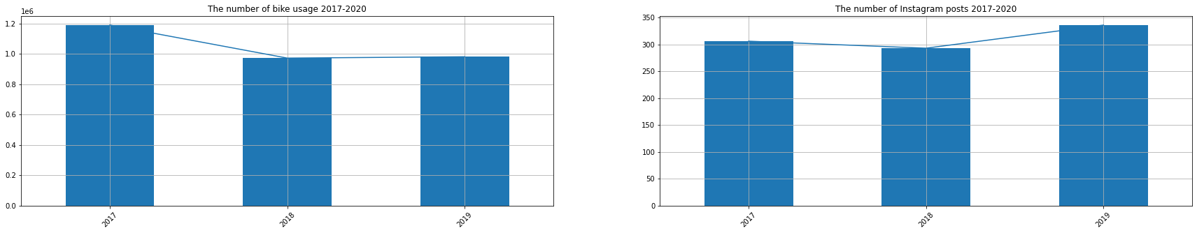
자전거 실제 사용 수는 줄었지만 인스타그램 게시물 수는 반대로 늘어가는 것을 볼 수 있습니다.
plt.figure(figsize=(20, 10))
plt.rc('font', size=15)

bike_bar_2017 = plt.subplot(231)
plt.tight_layout(pad=1.6)

bike_count_2017 = bike_2017['LEAS_YM']
bike_count_2017.plot(kind='bar', grid=True)
max_num_2017 = max(bike_count_2017)
min_num_2017 = min(bike_count_2017)

for i, count in enumerate(bike_count_2017):
    if count == max_num_2017:
        bike_bar_2017.get_children()[i].set_color("g")
    if count == min_num_2017:
        bike_bar_2017.get_children()[i].set_color("r")
plt.title("Year 2017 Usage")
plt.xlabel("Month")
plt.ylabel("number of usage")
plt.xticks(rotation=45)


bike_bar_2018 = plt.subplot(232)
plt.tight_layout(pad=1.6)

bike_count_2018 = bike_2018['LEAS_YM']
bike_count_2018.plot(kind='bar', grid=True)
max_num_2018 = max(bike_count_2018)
min_num_2018 = min(bike_count_2018)

for i, count in enumerate(bike_count_2018):
    if count == max_num_2018:
        bike_bar_2018.get_children()[i].set_color("g")
    if count == min_num_2018:
        bike_bar_2018.get_children()[i].set_color("r")
plt.title("Year 2018 Usage")
plt.xlabel("Month")
plt.ylabel("number of usage")
plt.xticks(rotation=45)


bike_bar_2019 = plt.subplot(233)
plt.tight_layout(pad=1.6)

bike_count_2019 = bike_2019['LEAS_YM']
bike_count_2019.plot(kind='bar', grid=True)
max_num_2019 = max(bike_count_2019)
min_num_2019 = min(bike_count_2019)

for i, count in enumerate(bike_count_2019):
    if count == max_num_2019:
        bike_bar_2019.get_children()[i].set_color("g")
    if count == min_num_2019:
        bike_bar_2019.get_children()[i].set_color("r")
plt.title("Year 2019 Usage")
plt.xlabel("Month")
plt.ylabel("number of usage")
plt.xticks(rotation=45)


bar_2017 = plt.subplot(234)
plt.tight_layout(pad=1.5)
count_2017 = count_YMD_2017
count_2017.plot(kind='bar', grid=True)
max_num_2017 = max(count_2017)
min_num_2017 = min(count_2017)

for i, count in enumerate(count_2017):
    if count == max_num_2017:
        bar_2017.get_children()[i].set_color("g")
    if count == min_num_2017:
        bar_2017.get_children()[i].set_color("r")
plt.title("Year 2017")
plt.xlabel("Month")
plt.ylabel("number of posts")
plt.xticks(rotation=45)

rects = bar_2017.patches

labels = count_2017

for rect, label in zip(rects, labels):
    height = rect.get_height()
    bar_2017.text(rect.get_x() + rect.get_width() / 2, height, label,
            ha='center', va='bottom')

bar_2018 = plt.subplot(235)
plt.tight_layout(pad=1.5)
count_2018 = count_YMD_2018
count_2018.plot(kind='bar', grid=True)
max_num_2018 = max(count_2018)
min_num_2018 = min(count_2018)

for i, count in enumerate(count_2018):
    if count == max_num_2018:
        bar_2018.get_children()[i].set_color("g")
    if count == min_num_2018:
        bar_2018.get_children()[i].set_color("r")
plt.title("Year 2018")
plt.xlabel("Month")
plt.ylabel("number of posts")
plt.xticks(rotation=45)

rects = bar_2018.patches

labels = count_2018

for rect, label in zip(rects, labels):
    height = rect.get_height()
    bar_2018.text(rect.get_x() + rect.get_width() / 2, height, label,
            ha='center', va='bottom')

bar_2019 = plt.subplot(236)
plt.tight_layout(pad=1.5)
count_2019 = count_YMD_2019
count_2019.plot(kind='bar', grid=True)
max_num_2019 = max(count_2019)
min_num_2019 = min(count_2019)

for i, count in enumerate(count_2019):
    if count == max_num_2019:
        bar_2019.get_children()[i].set_color("g")
    if count == min_num_2019:
        bar_2019.get_children()[i].set_color("r")

plt.title("Year 2019")
plt.xlabel("Month")
plt.ylabel("number of posts")
plt.xticks(rotation=45)

rects = bar_2019.patches

labels = count_2019

for rect, label in zip(rects, labels):
    height = rect.get_height()
    bar_2019.text(rect.get_x() + rect.get_width() / 2, height, label,
            ha='center', va='bottom')
월별로 확인해봅니다.
최소값은 붉은색, 최대값은 초록색으로 표시합니다.
9. 태그 정보로 워드 클라우드 그려보기
tags_df = pd.read_csv("./insta_tags_new.csv")
stop_tags = ['피프틴', 'fifteen', '피프틴자전거', '자전거', '고양시', '고양', 'bicycle', '선팔', '팔로우', '좋반', '좋아요반사',
             '고양시자전거', '자전거스타그램', 'follow', 'instadaily', '고양시공공자전거', '선팔하면맞팔']
tags = [ tag for tag in list(tags_df['tag']) if tag not in stop_tags]
cnt = Counter(tags)
most_100 = cnt.most_common(100)
태그 중에 필요없을 것으로 보이는 태그를 선정하고 해당 태그를 제외한 후
Counter를 활용해 각 태그를 카운팅 한 뒤
그 중 상위 빈도수 100번째 까지 남깁니다.
여기서 사용한 태그정보는 크롤링 시 따로 후처리 없이 사용할 수 있도록 저장한 데이터 입니다.
matplotlib.rcParams['font.family'] = "Maulgun Gothic"

wc = WordCloud(font_path=font_path, background_color="white", width=800, height=600)
cloud = wc.generate_from_frequencies(dict(most_100))
plt.figure(figsize = (20, 16))
plt.axis('off')
plt.imshow(cloud)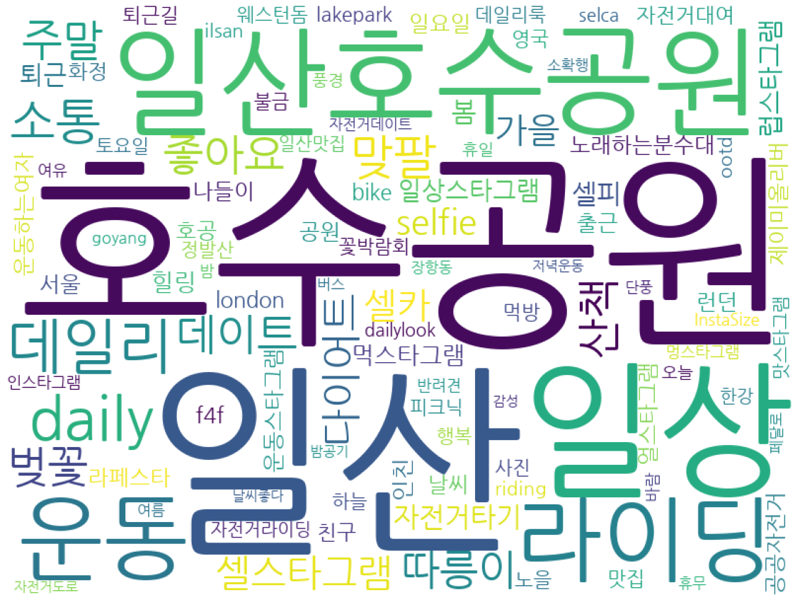
2012 ~ 2020년 사이의 태그 정보를 바탕으로 그린 워드클라우드를 보면
일산 호수공원이 가장 많이 등장하는 것을 볼 수 있습니다.
10. 각 년도 별로 그려보기
drop_duplicate_data['date_time_Y'] = drop_duplicate_data['date_time_YMD'].str.slice(0, 4)먼저 각 row 별 해당 데이터의 게시 년도를 추출합니다.
insta_data_2017 = drop_duplicate_data[drop_duplicate_data['date_time_Y'] == '2017']
insta_data_2018 = drop_duplicate_data[drop_duplicate_data['date_time_Y'] == '2018']
insta_data_2019 = drop_duplicate_data[drop_duplicate_data['date_time_Y'] == '2019']
insta_data_2020 = drop_duplicate_data[drop_duplicate_data['date_time_Y'] == '2020']
이를 바탕으로 각 년도로 데이터를 모아줍니다.
def get_tag_from_raw_data(text):
    tags = re.findall('#[A-Za-z0-9가-힣]+', text)
    tag = ''.join(tags).replace("#"," ") # "#" 제거

    tag_data = tag.split()

    return tag_data

def get_tags_from_main_text_and_comment(insta_data_df):
    upload_ids = list(insta_data_df['upload_id'])
    main_texts = list(insta_data_df['main_text'])
    comments = list(insta_data_df['comment'])

    instagram_tags = []

    for i in tqdm(range(len(main_texts))):
        tag_data = get_tag_from_raw_data(main_texts[i])

        for tag_one in tag_data:
            instagram_tags.append(tag_one)

        comment_dict = json.loads(comments[i])

        comment_keys = comment_dict.keys()

        for key in comment_keys:
            if comment_dict[key]['comment_id'] == upload_ids[i]:
                comment_text = comment_dict[key]['comment_text']

                tag_data = get_tag_from_raw_data(comment_text)

                for tag_one in tag_data:
                    instagram_tags.append(tag_one)

    return instagram_tags

def get_most_common_N(tag_list, N=100, stoptag=True):
    stop_tags = ['피프틴', 'fifteen', '피프틴자전거', '자전거', '고양시', '고양', 'bicycle', '선팔', '팔로우', '좋반', '좋아요반사',
                 '고양시자전거', '자전거스타그램', 'follow', 'instadaily', '고양시공공자전거', '선팔하면맞팔', '맞팔']
    if stoptag == False:
        stop_tags == []
    tags = [ tag for tag in tag_list if tag not in stop_tags]

    cnt = Counter(tags)
    most_100 = cnt.most_common(N)

    return most_100
- get_tag_from_raw_data(text):
=> 정규식을 활용하여 원본 text 중 #이 붙어있는 태그 정보만 추출하여 list 로 return
- get_tags_from_main_text_and_comment(insta_data_df):
=>크롤링 해온 데이터 중 원본과 댓글 데이터에서 태그 정보 추출하는 함수
=> 크롤링한 댓글 형식은 다음과 같습니다. ( json 형식 )
=> 게시물을 게시한 사람과 댓글을 작성한 사람들 중 게시물을 작성한 사람이 적은 댓글 속에 있는 태그 정보 추출
( 이렇게 작성한 이유는 게시물 원본 글에 태그를 적지 않고 댓글에 적는 사용자도 있기 때문 )
{'1': {'comment_id': 'comment_id', 'comment_text': '헐 노리 완전기여워용😍'},
 '2': {'comment_id': 'comment_id', 'comment_text': '노리 재밌었겠다 ㅋㅋ'},
 '3': {'comment_id': 'comment_id', 'comment_text': '민턴맞팔해요^^'},
 '4': {'comment_id': 'comment_id', 'comment_text': '노리근데 머리 뭐 낫어 벗겨짐?!!!'},
 '5': {'comment_id': 'comment_id',
  'comment_text': '@jaengtori 응 늙어서.. 실제로 와서 바바....😭'},
 '6': {'comment_id': 'comment_id', 'comment_text': '긁은거 아녀?!!!!'}}
- get_most_common_N(tag_list, N=100, stoptag=True):
=> 빈도수 상위 N 번째 까지의 태그 정보를 가져옴
=> stoptag를 True로 설정하면 필요 없는 미리 설정한 태그는 제외합니다.
tags_2017 = get_tags_from_main_text_and_comment(insta_data_2017)
tags_2018 = get_tags_from_main_text_and_comment(insta_data_2018)
tags_2019 = get_tags_from_main_text_and_comment(insta_data_2019)
tags_2020 = get_tags_from_main_text_and_comment(insta_data_2020)
이를 바탕으로 2017년 ~ 2020년 각 년도별 태그를 추출합니다.
plt.figure(figsize = (360, 120))
plt.rc('font', size=100)

plt.subplot(411)
most_2017 = get_most_common_N(tags_2017)
wc_2017 = WordCloud(font_path=font_path, background_color="white", width=1200, height=400)
cloud_2017 = wc_2017.generate_from_frequencies(dict(most_2017))
plt.title("Year 2017")
plt.imshow(cloud_2017)

plt.subplot(412)
most_2018 = get_most_common_N(tags_2018)
wc_2018 = WordCloud(font_path=font_path, background_color="white", width=1200, height=400)
cloud_2018 = wc_2018.generate_from_frequencies(dict(most_2018))
plt.title("Year 2018")
plt.imshow(cloud_2018)

plt.subplot(413)
most_2019 = get_most_common_N(tags_2019)
wc_2019 = WordCloud(font_path=font_path, background_color="white", width=1200, height=400)
cloud_2019 = wc_2019.generate_from_frequencies(dict(most_2019))
plt.title("Year 2019")

plt.imshow(cloud_2019)

plt.subplot(414)
most_2020 = get_most_common_N(tags_2020)
wc_2020 = WordCloud(font_path=font_path, background_color="white", width=1200, height=400)
cloud_2020 = wc_2020.generate_from_frequencies(dict(most_2020))
plt.title("Year 2020")

plt.imshow(cloud_2020)
모든 년도에 호수공원이 가장 빈도수가 높은 태그로 등장하는 것을 볼 수 있습니다.
그 이외에도 일요일, 주말, 데이트 등 다양한 태그가 등장하는 것을 볼 수 있었습니다.
읽어주셔서 감사합니다.
'경진대회, 공모전 > COMPAS 고양시 공공자전거 스테이션 최적 위치 선정' 카테고리의 다른 글
| python 카테고리 나누기 / pydeck을 이용하여 스테이션별 이용량 파악하기 (0) | 2020.09.11 |
|---|---|
| python boxplot을 통해 데이터 빈도 알아보기/ 고양시 운영이력 데이터 살펴보기 (0) | 2020.09.11 |
| [COMPAS 고양시] 데이터 시각화 해보기 ( feat. python, folium ) (0) | 2020.08.01 |